JEasyTFM - User manual (pdf version)


JEasyTFM - Input and output files and folders names and formats (pdf version)

Technical requirements for the use of JeasyTFM


JEasyTFM - User manual (pdf version) [top]


Fully functional bundle: To use the fully functional ImageJ bundle, just download the platform-dependent version of ImageJ bundled with Java file and containing all the tools needed for the package embedded:
  • ImageJ bundled with Java 8 and JEasyTFM under 64-bit Windows
  • ( 80.6 Mb)
  • ImageJ bundled with Java 8 and JEasyTFM under 64-bit Linux
  • ( 79.6 Mb)
  • ImageJ bundled with Java 8 and JEasyTFM under 64-bit Mac
  • (120 Mb)
  • ImageJ bundled with Zulu OpenJDK 13.0.6. and JEasyTFM under 64-bit Mac
  • ( 88 Mb)
    By unzipping and launching ImageJ, there will a JEasyTFM command at the right of the ImageJ menu for using it.
    ImageJ window
    or

    Manual installation: Proceed with the manual installation by downloading the ImageJ software and unziping it.
    Check wether the given ImageJ version is 1.54f11 or higher and if not replace the ij.jar file with its daily-build version.

    Download JEasy_TFM.jar to the plugins/jars folder, restart ImageJ, and there will a JEasyTFM new command at the right of the ImageJ menu.
    But in order to be fully fonctional, the JEasyTFM package uses several third party open source plugins which origin will be indicated next to the needed tool.
    Nevertheless, most of the linked plugins have been modified (with at least the the addition of some "direct static methods") and very often improved with the addition of new functionalities and features.
    All the modified source codes are available inside the jar files for further editing and improvements.
    Thus the following additional tools need to be downloaded from the links below (and not the original sites) to the plugins/jars folder:

  • the Particle Tracker PIV and Trajectories Inputs
  • plugin which is an improved version of the ParticleTracker_2D plugin from the MOSAIC group at the Systems Biology Dresden (CSBD).
  • the MosaicSuite-1.0.25_Full_extended
  • package which is an improved version of the MosaicSuite 1.0.25 package from the MOSAIC group at the Systems Biology Dresden (CSBD),
  • the Extended Depth of Field
  • plugin from the Biomedical Imaging Group at EPFL,
  • the Template Matching and Slice Alignment
  • plugin from the Qingzong Tseng website,
  • the Find Focused Slices
  • plugin from the Qingzong Tseng website,
  • the PIV (Particle Image Velocimetry)
  • plugin from the Qingzong Tseng website,
  • the Traction Force Microscopy
  • plugin from the Qingzong Tseng website,
  • the Apache Commons Mathematics
  • library file,
  • some of the previous plugins require the javacv
  • library files: javacv.jar, javacpp.jar, opencv.jar.

    Alternatively the download of all the previously described files can simply be replaced by downloading the JEasyTFM_files file and unzip it in the plugins/jars folder.

    Finally one of the platform-dependent library files need to be downloaded into the plugins/jars folder:
  • 32-bit Windows
  • 64-bit Windows
  • 64-bit Mac
  • 32-bit Linux
  • 64-bit Linux
  • The JEasyTFM tool is divided into two submenus:

    JEasyTFM Create job
    • JEasyTFM>Create_job - for setting up the analysis configuration job, the data of which will then be saved into a batch file (JEasy.txt) within the ImageJ plugins folder.
    • JEasyTFM>Launch_job - will be reading the generated batch file (JEasy.txt) and launch the analysis job it defines.

    Splitting the JEasyTFM tool into two steps, with on one side a job creation and on the other side, a job launching operation, provides two main advantages. The first one is to offer traceability of all the analysis settings used to generate the different analysis results. In the case of heavily booked dedicated analysis computers, the second one is to rapidly define and protect the analysis settings, which can then quickly be launched later on once the machine is available.

    When launching the JEasyTFM->Create_job tab, the following window will be displayed:

    Create_job_GUI Debug Data Folder Sequence images Reference images Number of acquired cells Slices Frames Frames begin Beads1 Beads2 Ch1 Ch2 Ch3 Number of Ch Kurto1 Kurto2 Kurto3 Young's modulus Precision_for_the_Regularization_factor_calculation Cells images Cells starting folder Cells ending folder image chosen from slices Beads reference images Beads reference starting folder Beads reference ending folder Beads reference images find focused slices Beads sequence images Beads sequence starting folder Beads sequence ending folder Beads sequence images find focused slices Traction force Traction starting folder Traction ending folder Traction force alignment Alignment make Alignment crop Traction force calculation PIV calculation Lambda calculation Force calculation Force superposition Cells analysis Cells analysis starting folder Cells analysis ending folder Cells selection Cells segmentation Force integration Traction high force Traction high starting folder Traction high ending folder Traction high enhance contrast High PIV calculation Particle tracker FA segmentation FA segmentation starting folder FA segmentation ending folder Traction force applied on FA Traction force applied on FA starting folder Traction force applied on FA ending folder Generate file and Exit Cancel
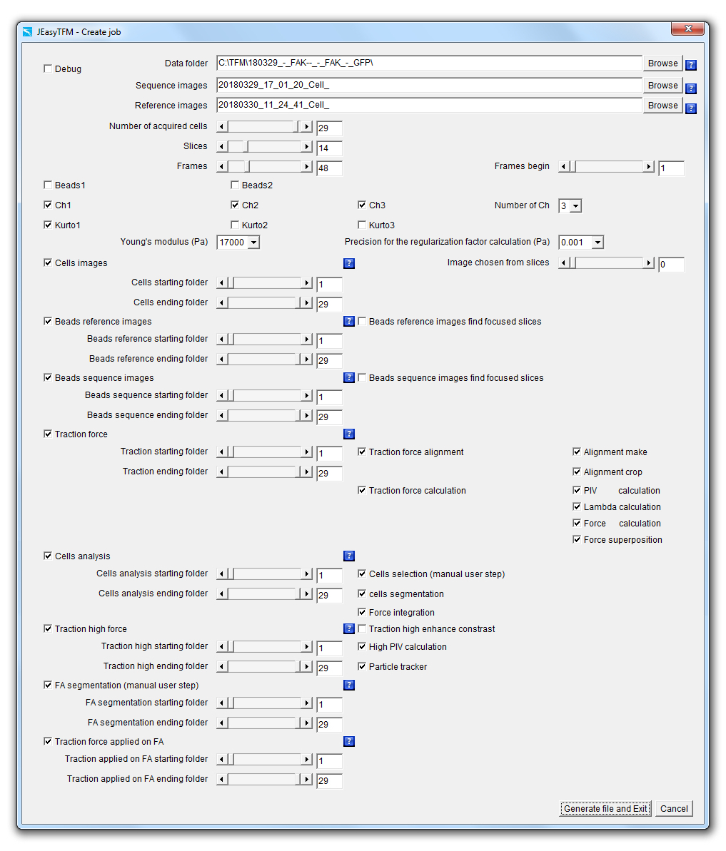
    We will now explain each point in details.
    Data folder and file names definitions Debug Data Folder Sequence images Reference images

    Debug: When the Debug checkbox is selected, the analysis is performed by launching the different used plugins going through their GUI, often resulting in images being displayed at each stage for the user to visualize the results of the different processes going on. On the contrary, when the Debug checkbox is unselected, all the analyses are performed launching the additional plugins by using some back-doors (i.e. static methods) that have been created to short-cut the plugins GUI resulting in all the images produced in memory and not displayed for a gain of machine time.

    Data_folder: On clicking on the Data_folder Browse button, a "choose directory" dialog is displayed for the user to choose the directory in which the data to be analyzed are saved. Upon selection validation of the chosen folder, its path will be updated within the field Data_folder together with the prefixes file name of the acquired images to be analyzed in the File field and the one for the images of the beads at equilibrium (i.e. after the addition of trypsin also called reference images in this document) in the Reference_images field.
    Note that it is also possible to populate the different texts fields (i.e. the Data_folder, File and Reference_images fields) with a simple Drag&Drop of an image file in the field Data_folder.

    Sequence_images: On clicking on the Sequence_images Browse button, a "file open" dialog is displayed for the user to choose an image file to be analyzed. Upon selection validation of an image file, the file name prefix of the acquired images to be analyzed will be updated within the Sequence_images field.
    Note that it is also possible to populate the Sequence_images field with a simple Drag&Drop of an image file in the field.

    Reference_images: On clicking on the Reference_images Browse button, a "file open" dialog is displayed for the user to choose a reference images file to be analyzed. Upon selection validation of the image file, the file name prefix of the acquired images to be analyzed will be updated within the Reference_images field. The reference images selected in Reference_images have to be previously saved within a folder whose name is the one defined within Data_folder field with the addition of "_-_Reference".
    Note that it is also possible to populate the Reference_images field with a simple Drag&Drop of an image file in the field.

    Sizes definitions Number of acquired cells Slices Frames Frames begin

    Number_of_acquired_cells: Slider defining the number of cells that have been recorded during the acquisitions.
    Note that the value specified by the Number_of_acquired_cells slider represents the maximum value for the sliders: Note that all the sliders values within JEasyTFM>Create_job can either be modified directly by a mouse drag, by using the arrow or page-Up/page-Down keys or by typing in the value within the numeric field, but also with a mouse wheel on top of the slider or within the numeric field.

    Slices: Slider defining the number of z-slices that have been acquired during the acquisitions.
    Note that the setting of this field is ignored in the case the source images are saved in the form of hyperstacks in which case the image z-slices properties are taken into account.

    Frames: Slider defining the number of time-frames that have been acquired during the acquisitions.
    Note that the setting of this field is ignored in the case the source images are saved in the form of hyperstacks in which case the image time-frames properties are taken into account.

    Frames_begin: Slider whose maximum value will be defined by the Frames slider and defining the first time-frames number of the data that will be analyzed.
    This option can be used in the case an analysis process has been canceled before completion to not have to restart the analysis from the first frame.

    Experiment definition Beads1 Beads2 Ch1 Ch2 Ch3 Number of Ch Kurto1 Kurto2 Kurto3 Young's modulus Precision_for_the_Regularization_factor_calculation

    Beads1: The selection of the Beads1 and/or Beads2 checkboxes implies that an experiment of high-resolution TFM has been performed, i.e. with the use of beads with two different colors.
    Under the high-resolution TFM configuration, the selection of the Beads1 checkbox will enable the analysis of the data with the beads of color 1.
    Note that in the case of the analysis of "regular" TFM experiments, i.e. with the use of a single color, it is easier to proceed with the analysis without selecting any of the Beads1 or Beads2 checkboxes.

    Beads2: The selection of the Beads2 and/or Beads1 checkboxes implies that an experiment of high-resolution TFM has been performed, i.e. with the use of beads with two different colors.
    Under the high-resolution TFM configuration, the selection of the Beads2 checkbox will enable the analysis of the data with the beads of color 2.
    Note that in the case of the analysis of "regular" TFM experiments, i.e. with the use of a single color, it is easier to proceed with the analysis without selecting any of the Beads1 or Beads2 checkboxes.

    Ch1: The selection of the Ch1 and/or Ch2 and/or Ch3 checkboxes implies that more than one channel has been acquired for imaging the cells.
    Under these acquisitions conditions, the selection of the Ch1 checkbox will enable the analysis of the data of the first channel (for example a Bright Field channel).
    Note that in the case of the analysis of an experiment where only one channel has been acquired for imaging the cells, it is easier to proceed with the analysis without selecting any of the Ch1, Ch2 or Ch3 checkboxes.
    Note also that Ch1, Ch2 and Ch3 may correspond to any cell channel being recorded.

    Ch2: The selection of the Ch1 and/or Ch2 and/or Ch3 checkboxes implies that more than one channel has been acquired for imaging the cells.
    Under these acquisitions conditions, the selection of the Ch1 checkbox will enable the analysis of the data of the second channel (for example an Epifluorescence channel).
    Note that in the case of the analysis of an experiment where only one channel has been acquired for imaging the cells, it is easier to proceed with the analysis without selecting any of the Ch1, Ch2 or Ch3 checkboxes.
    Note also that Ch1, Ch2 and Ch3 may correspond to any cell channel being recorded.

    Ch3: The selection of the Ch1 and/or Ch2 and/or Ch3 checkboxes implies that more than one channel has been acquired for imaging the cells.
    Under these acquisitions conditions, the selection of the Ch1 checkbox will enable the analysis of the data of the third channel (for example a channel corresponding to a Hoechst staining).
    Note that in the case of the analysis of an experiment where only one channel has been acquired for imaging the cells, it is easier to proceed with the analysis without selecting any of the Ch1, Ch2 or Ch3 checkboxes.
    Note also that Ch1, Ch2 and Ch3 may correspond to any cell channel being recorded.

    Number of Ch: Popup menu defining the number of channels that have been acquired.
    When selecting 2 channels within the Number of Ch popup menu, the Ch3 checkbox will be hidden.
    And when selecting only 1 channel within the Number of Ch popup menu, the Ch1, Ch2 and Ch3 checkboxes will be hidden.

    Kurto1: The Kurto1 checkbox will apply a best Kurtosis selection algorithm to the images of the Ch1 in the case it is selected and the "Extended Depth Field"1 plugin in the case it is unselected.
    Note that the Kurtosis algorithm should rather be applied on images of a Bright Field channel as the "Extended Depth Field" on images of a fluorescent channel.

    Kurto2: The Kurto2 checkbox will apply a best Kurtosis selection algorithm to the images of the Ch2 in the case it is selected and the "Extended Depth Field"1 plugin in the case it is unselected.
    Note that the Kurtosis algorithm should rather be applied on images of a Bright Field channel as the "Extended Depth Field" on images of a fluorescent channel.

    Kurto3: The Kurto3 checkbox will apply a best Kurtosis selection algorithm to the images of the Ch3 in the case it is selected and the "Extended Depth Field"1 plugin in the case it is unselected.
    Note that the Kurtosis algorithm should rather be applied on images of a Bright Field channel as the "Extended Depth Field" on images of a fluorescent channel.

    Young's_modulus_Pa: Numerical field defining the Young's modulus in Pascal units of the support used for cell plating.

    Precision_for_the_Regularization_factor_calculation: Popup menu defining the precision for the calculation of the regularization or Lagrange parameter λ value that is used to convert the measured beads displacements to the forces applied from the cells onto their support.
    The regularization or Lagrange parameter λ value determination is performed by using a binary search algorithm.

    (1) Forster, B., Van De Ville, D., Berent, J., Sage, D. & Unser, M. Complex Wavelets for Extended Depth-of-Field: A New Method for the Fusion of Multichannel Microscopy Images. Microsc. Res. Tech. 65, 33-42 (2004).
    Cells images extraction Cells images Cells starting folder Cells ending folder image chosen from slices
    The Cells_images analysis will create a folder for each cell number defined within Cells_starting_folder and Cells_ending_folder within which all following analysis data will be saved.

    Cells_images: The checkbox defines whether cell images should be extracted from all the Slices for all the defined Frames and for the cells numbers defined between the Cells_starting_folder and Cells_ending_folder.
    If the checkboxes Ch1 and/or Ch2 and/or Ch3 is/are activated, this extraction will then be applied to all the selected channels.

    Cells_starting_folder: Defines the first cell number or folder for which cell images should be extracted from all the Slices and for all the defined Frames.
    If the checkboxes Ch1 and/or Ch2 and/or Ch3 is/are activated, this extraction will then be applied to all the selected channels.

    Cells_ending_folder: Defines the last cell number or folder for which cell images should be extracted from all the Slices and for all the defined Frames.
    If the checkboxes Ch1 and/or Ch2 and/or Ch3 is/are activated, this extraction will then be applied to all the selected channels.

    Image_chosen_from_slices: The automatic selection of the best focused image may be performed by putting the value 0 in this slider. In this case, a Kurtosis algorithm will be applied on the Slices images in order to extract the one giving the highest value and this for all the defined Frames. On the other hand, manual inspection of the z-slices can be performed and the slice number of the selected best focused image can be defined in the Image_chosen_from_slices slider by choosing which cell image number between 1 and the number indicated in Slices should be extracted from all the Slices for all the defined Frames.

    Beads reference images best focus extraction Beads reference images Beads reference starting folder Beads reference ending folder Beads reference images find focused slices

    Beads_Reference_images: The checkbox defines whether images corresponding to the best focused image of the beads extracted within the z-series acquired with the support at equilibrium (i.e. after the cells have been detached from the surface) should be extracted from all the Slices.
    If the checkboxes Beads1 and/or Beads2 is/are activated, this extraction will then be applied to all the selected beads colors.

    Beads_reference_starting_folder: Defines the first cell number or folder for which images corresponding to the best focus of the beads within the images acquired with the support at equilibrium (i.e. after the cells have been detached from the surface) should be extracted from all the Slices.
    If the checkboxes Beads1 and/or Beads2 is/are activated, this extraction will then be applied to all the selected beads colors.

    Beads_reference_ending_folder: Defines the last cell number or folder for which images corresponding to the best focus of the beads within the images acquired with the support at equilibrium (i.e. after the cells have been detached from the surface) should be extracted from all the Slices.
    If the checkboxes Beads1 and/or Beads2 is/are activated, this extraction will then be applied to all the selected beads colors.

    Beads_Reference_images_find_focused_slices: The checkbox defines whether the "Find focused slices"2 plugin should be applied prior to applying the "Extended Depth Field"1 plugins on the images of the beads with the support at equilibrium from all the Slices in order to extract the best focused image.
    This option can be activated in order to reduce the number of images used as input for the "Extended Depth Field" plugin in the case its output is too noisy for the rest of the analysis to be completed.

    (2) Tseng, Q. Find Focused Slices. ImageJ plugin available at: https://sites.google.com/site/qingzongtseng/find-focus
    (1) Forster, B., Van De Ville, D., Berent, J., Sage, D. & Unser, M. Complex Wavelets for Extended Depth-of-Field: A New Method for the Fusion of Multichannel Microscopy Images. Microsc. Res. Tech. 65, 33–42 (2004).
    Beads sequence images best focus extraction Beads sequence images Beads sequence starting folder Beads sequence ending folder Beads sequence images find focused slices

    Beads_Sequence_images: The checkbox defines whether images corresponding to the best focus of the beads extracted within the images through the acquired time-lapse should be extracted from all the Slices for all the defined Frames.
    If the checkboxes Beads1 and/or Beads2 is/are activated, this extraction will then be applied to all the selected beads colors.

    Beads_sequence_starting_folder: Defines the first cell number or folder for which images corresponding to the best focus of the beads extracted within the images through the acquired time-lapse should be extracted from all the Slices for all the defined Frames.
    If the checkboxes Beads1 and/or Beads2 is/are activated, this extraction will then be applied to all the selected beads colors.

    Beads_sequence_ending_folder: Defines the last cell number or folder for which images corresponding to the best focus of the beads extracted within the images through the acquired time-lapse should be extracted from all the Slices for all the defined Frames.
    If the checkboxes Beads1 and/or Beads2 is/are activated, this extraction will then be applied to all the selected beads colors.

    Beads_Sequence_images_find_focused_slices: The checkbox defines whether the "Find focused slices"2 plugin should be applied prior to applying the "Extended Depth Field"1 plugin on the images of the beads through the acquired time-lapse, defining the Frames from all the Slices for all the defined Frames to extract the best focused image.
    This option can be activated in order to reduce the number of images used as input for the "Extended Depth Field" plugin in the case its output is too noisy for the rest of the analysis to be completed.

    (2) Tseng, Q. Find Focused Slices. ImageJ plugin available at: https://sites.google.com/site/qingzongtseng/find-focus
    (1) Forster, B., Van De Ville, D., Berent, J., Sage, D. & Unser, M. Complex Wavelets for Extended Depth-of-Field: A New Method for the Fusion of Multichannel Microscopy Images. Microsc. Res. Tech. 65, 33–42 (2004).
    Traction force analysis Traction starting folder Traction force Traction ending folder Traction force alignment Alignment make Alignment crop Traction force calculation PIV calculation Lambda calculation Force calculation Force superposition

    Traction_force: The checkbox defines whether the whole or part of the force calculation processes should be launched.
    This is the main checkbox for the analysis, which means that if it is not selected, none of the following analysis processes: will be launched whether or not they are selected.
    If the checkboxes Beads1 and/or Beads2 is/are activated, the launched analysis will then be applied to all the selected beads colors.

    Traction_starting_folder: Defines the first cell number or folder for which the whole or part of the force calculation processes should be calculated.
    If the checkboxes Beads1 and/or Beads2 is/are activated, this calculation will then be applied to all the selected beads colors.

    Traction_ending_folder: Defines the last cell number or folder for which the whole or part of the force calculation processes should be calculated.
    If the checkboxes Beads1 and/or Beads2 is/are activated, this calculation will then be applied to all the selected beads colors.

    Traction_force_alignment: The checkbox defines whether the whole or part of the images alignment processes should be calculated.
    This means that if the checkbox Traction_force_alignment is not selected none of the following images alignment processes: will be launched whether or not they are selected.
    If the checkboxes Beads1 and/or Beads2 is/are activated, the launched analysis will then be applied to all the selected beads colors.

    Alignment_make: The checkbox defines whether an alignment algorithm should be launched on the images.
    This algorithm consists of applying the "Template Matching and Slice Alignment"3 plugin on all the images that have been previously generated with the Beads_Sequence_images feature (that correspond to the best focused images of the beads extracted from all the Slices for all the defined Frames) taking as reference the image that has been previously generated with the Beads_Reference_images feature (that correspond to the best focused images of the beads extracted with the support at equilibrium, i.e. after the cells have been detached from the surface) and this for all the defined Frames.
    Once the alignment is performed on the images of the beads, the obtained displacement is then applied on all the selected channel images Ch1 and/or Ch2 and/or Ch3.
    If the checkboxes Beads1 and/or Beads2 is/are activated, this algorithm will then be applied to all the selected beads colors.
    Note that the Alignment_make feature will only be launched if the Alignment_make, Traction_force_alignment and Traction_force checkboxes are all selected.
    (3) Tseng, Q. Find Focused Slices. ImageJ plugin available at: https://sites.google.com/site/qingzongtseng/template-matching-ij-plugin.

    Alignment_crop: The checkbox defines whether the algorithm that will get rid of the image borders generated by the Alignment_make algorithm should be launched on the images.
    The algorithm automatically detects the maximum displacement during image alignment through all the defined Frames and applies cropping on the defined region.
    Once the cropping is performed on the images of the beads, the obtained border selection and cropping is then applied on all the selected channel images Ch1 and/or Ch2 and/or Ch3.
    If the checkboxes Beads1 and/or Beads2 is/are activated, this cropping will then be applied to all the selected beads colors.
    Note that the Alignment_crop feature will only be launched if the Alignment_crop, Traction_force_alignment and Traction_force checkboxes are all selected.

    Traction_force_calculation: The checkbox defines whether the whole or part of the images forces calculation processes should be launched.
    This means that if the checkbox Traction_force_calculation is not selected none of the following force calculation processes: will be launched whether or not they are selected.
    If the checkboxes Beads1 and/or Beads2 is/are activated, the launched analysis will then be applied to all the selected beads colors.

    PIV_calculation: The checkbox defines whether a PIV (Particle Image Velocimetry) algorithm should be launched on the images of the aligned and cropped beads in order to generate beads displacement maps.
    This algorithm consists of applying the "PIV (Particle Image Velocimetry)"4 plugin on all the images of the beads that have been previously aligned and cropped with the Alignment_make and Alignment_crop algorithms taking as reference the image of the beads with the support at equilibrium and this for all the defined Frames.
    The displacement vectors spacing of the generated displacement map images is of 16 pixels, which in the case of a camera pixel size of 6.5 μm and a used objective magnification of 60× corresponds to 1.733 μm.
    If you are using a camera system for which the pixel size isn't equal to 6.5 µm, or the objective magnification equal to 60×, then these values have to be modified manually within the job file "JEasyTFM.txt" (saved in the "ImageJ/plugins" folder) and more precisely the 2 first lines of the file designed by camera_pixel_size and objective_magnification.
    If the checkboxes Beads1 and/or Beads2 is/are activated, this algorithm will then be applied to all the selected beads colors.
    Note that the PIV_calculation feature will only be launched if the PIV_calculation, Traction_force_calculation and Traction_force checkboxes are all selected.
    (4) Tseng, Q. PIV (Particle Image Velocimetry). ImageJ plugin available at: https://sites.google.com/site/qingzongtseng/piv.

    Lambda_calculation: The checkbox defines whether the regularization or Lagrange parameter λ values should be calculated.
    This algorithm consists of using a binary search algorithm to calculate the regularization or Lagrange parameter λ values for the different frames.
    The regularization or Lagrange parameter λ values will be used within the Force_calculation analysis step to convert the beads displacement maps previously generated with the PIV_calculation feature into force maps by using an a Fourier Transform Traction Cytometry (FTTC) algorithm.
    If the checkboxes Beads1 and/or Beads2 is/are activated, this algorithm will then be applied to all the selected beads colors.
    Note that the Lambda_calculation feature will only be launched if the Lambda_calculation, Traction_force_calculation and Traction_force checkboxes are all selected.

    Force_calculation: The checkbox defines whether a Fourier Transform Traction Cytometry (FTTC) algorithm should be launched on the beads displacement maps previously generated with the PIV_calculation feature in order to create force maps.
    This algorithm consists of applying the "Traction Force Microscopy"5 plugins on all the PIV data that have been previously generated with the PIV_calculation algorithm and this for all the defined Frames.
    If the checkboxes Beads1 and/or Beads2 is/are activated, this algorithm will then be applied to all the selected beads colors.
    Note that the Force_calculation feature will only be launched if the Force_calculation, Traction_force_calculation and Traction_force checkboxes are all selected.
    (5) Tseng, Q. Traction Force Microscopy. ImageJ plugin available at: https://sites.google.com/site/qingzongtseng/tfm.

    Force_superposition: The checkbox defines whether the force maps previously generated with the Force_calculation feature should be superimposed with the images of the cells that have been previously generated with the Cells_images feature.
    If the checkboxes Ch1 and/or Ch2 and/or Ch3 is/are activated, this superimposition will then be applied to all the selected channels.
    If the checkboxes Beads1 and/or Beads2 is/are activated, this extraction will also be applied to all the selected beads colors.
    Note that the Force_superposition feature will only be launched if the Force_superposition, Traction_force_calculation and Traction_force checkboxes are all selected.

    Cells analysis Cells analysis Cells analysis starting folder Cells analysis ending folder Cells selection Cells segmentation Force integration

    Cells_analysis: The checkbox defines whether the whole or part of the cells segmentation and force integration processes should be launched. This is the main checkbox for the analysis, which means that if it is not selected none of the following analysis processes: will be launched whether or not they are selected.
    If the checkboxes Beads1 and/or Beads2 is/are activated, the launched analysis will then be applied to all the selected beads colors.

    Cells_analysis_starting_folder: Defines the first cell number or folder for which the whole or part of the cells segmentation and force integration processes should be launched.
    If the checkboxes Beads1 and/or Beads2 is/are activated, this algorithm will then be applied to all the selected beads colors.

    Cells_analysis_ending_folder: Defines the last cell number or folder for which the whole or part of the cells segmentation and force integration processes should be launched.
    If the checkboxes Beads1 and/or Beads2 is/are activated, this algorithm will then be applied to all the selected beads colors.

    Cells_selection (manual user step): The checkbox defines whether a cells segmentation algorithm with some manual user steps should be launched on the images of the cells that have been previously aligned and cropped with the Alignment_make and Alignment_crop algorithms and pre-filtered with the Cells_segmentation algorithm.
    This part of the algorithm consist of manually defining some cells border as well as threshold settings which will then be applied for all the Frames images on all the images of the cells that have been previously aligned and cropped with the Alignment_make and Alignment_crop algorithms and filtered with the Cells_segmentation algorithm.
    If the checkboxes Beads1 and/or Beads2 is/are activated, the filter application algorithm will then be applied to all the selected beads colors.
    Note that the Cells_selection (manual user step) feature will only be launched if the Cells_analysis checkbox is selected as well.

    Cells_segmentation: The checkbox defines whether a cells segmentation algorithm should be launched on the images of the cells that have been previously aligned and cropped with the Alignment_make and Alignment_crop algorithms.
    The cells segmentation algorithm is split in two, given that it implies some user action.
    This part of the algorithm consist of applying different image filters on all the images of the cells that have been previously aligned and cropped with the Alignment_make and Alignment_crop algorithms and this for all the defined Frames.
    If the checkboxes Beads1 and/or Beads2 is/are activated, the filter application algorithm will then be applied to all the selected beads colors.
    Note that the Cells_segmentation feature will only be launched if the Cells_analysis checkbox is selected as well.

    Force_integration: The checkbox defines whether a whole cells force integration algorithm should be launched on the traction force images using the cells segmentation ROI (Region Of Interest) data that have been obtained either automatically through a Cells_selection (manual user step) algorithm or manually and the result together with the ROI drawing superimposed with the images of the cells that have been previously generated with the Cells_images feature.
    If the checkboxes Ch1 and/or Ch2 and/or Ch3 is/are activated, this superimposition will then be applied to all the selected channels.
    If the checkboxes Beads1 and/or Beads2 is/are activated, the filter application algorithm will then be applied to all the selected beads colors.
    Note that the Force_integration feature will only be launched if the Cells_analysis checkbox is selected as well.

    Beads positions tracking Traction high force Traction high starting folder Traction high ending folder Traction high enhance contrast High PIV calculation Particle tracker

    Traction_high_force: The checkbox defines whether the whole or part of the beads positions tracking processes should be launched.
    This is the main checkbox for the analysis, which means that if it is not selected none of the following analysis processes: will be launched whether or not they are selected.
    If the checkboxes Beads1 and/or Beads2 is/are activated, the launched analysis will then be applied to all the selected beads colors.

    Traction_high_starting_folder: Defines the first cell number or folder for which the whole or part of the beads positions tracking processes should be calculated.
    If the checkboxes Beads1 and/or Beads2 is/are activated, this algorithm will then be applied to all the selected beads colors.

    Traction_high_ending_folder: Defines the last cell number or folder for which the whole or part of the beads positions tracking processes should be calculated.
    If the checkboxes Beads1 and/or Beads2 is/are activated, this algorithm will then be applied to all the selected beads colors.

    Traction_high_enhance_contrast: The checkbox defines whether a Subtract_Background... followed by an Enhance_Contrast... filter should be applied on the images in order to enhance their contrast before applying the High_PIV_calculation regression.
    Note that the Traction_high_enhance_contrast feature will only be launched if the Traction_high_force checkbox is selected as well.

    High_PIV_calculation: The checkbox defines whether a PIV (Particle Image Velocimetry) algorithm should be launched on the images of the aligned and cropped beads in order to generate beads displacement maps.
    This algorithm consists of applying the "PIV (Particle Image Velocimetry)"4 plugin on all the images of the beads that have been previously aligned and cropped with the Alignment_make and Alignment_crop algorithms taking as reference the image of the beads with the support at equilibrium and this for all the defined Frames.
    The difference between the High_PIV_calculation and the PIV_calculation is that the displacement vectors spacing of the generated displacement map images are now pushed up to 8 pixels, and the calculation starts with the results of the 16 pixels displacement vectors spacing maps which have previously been obtained from the PIV_calculation algorithm.
    The reason why we are pushing the displacement vectors spacing of the generated displacement maps from 16 to 8 pixels is that this precision is needed in order to get consistent results with the tracking algorithm used in the next step.
    For information, a displacement vectors spacing of the generated force maps images of 8 pixels corresponds to 0.866 μm in the case of a camera pixel size of 6.5 μm and a used objective magnification of 60×.
    If the checkboxes Beads1 and/or Beads2 is/are activated, this algorithm will then be applied to all the selected beads colors.
    Note that the High_PIV_calculation feature will only be launched if the Traction_high_force checkbox is selected as well.
    (4) Tseng, Q. PIV (Particle Image Velocimetry). ImageJ plugin available at: https://sites.google.com/site/qingzongtseng/piv.

    Particle_tracker: The checkbox defines whether a particle tracking algorithm should be launched on the beads displacement maps previously generated with the High_PIV_calculation feature in order to track the beads displacements between images that have been previously generated with the Beads_Sequence_images.
    The beads tracking algorithm used on the images data is an improvement of the ParticleTracker_2D6 plugin which have initially been developed by the Mosaic group (http://mosaic.mpi-cbg.de/ParticleTracker/index.html).
    The new additions consist essentially of giving the possibility to input the beads displacement vector maps that have been previously generated with the High_PIV_calculation algorithm as a starting position for the particle linking algorithm as well as giving the possibility to reload and manually correct the trajectories obtained by the algorithm.
    If the checkboxes Beads1 and/or Beads2 is/are activated, this generation will then be applied to all the selected beads colors.
    Note that the Particle_tracker feature will only be launched if the Traction_high_force checkbox is selected as well.
    (6) Sbalzarini, I. F. & Koumoutsakos, P. Feature point tracking and trajectory analysis for video imaging in cell biology. J. Struct. Biol. 151, 182–195 (2005).


    FA segmentation FA segmentation FA segmentation starting folder FA segmentation ending folder

    FA_segmentation (manual user step): The checkbox defines whether a FA_segmentation (manual user step) algorithm should be launched on fluorescent images of the cells that have been previously aligned and cropped with the Alignment_make and Alignment_crop algorithms.
    If the checkboxes Beads1 and/or Beads2 is/are activated, this algorithm will then be applied to all the selected beads colors.

    FA_segmentation_starting_folder: Defines the first cell number or folder for which the FA_segmentation (manual user step) algorithm should be applied.
    If the checkboxes Beads1 and/or Beads2 is/are activated, this algorithm will then be applied to all the selected beads colors.

    FA_segmentation_ending_folder: Defines the last cell number or folder for which the FA_segmentation (manual user step) algorithm should be applied.
    If the checkboxes Beads1 and/or Beads2 is/are activated, this algorithm will then be applied to all the selected beads colors.

    Traction force applied on FA Traction force applied on FA Traction force applied on FA starting folder Traction force applied on FA ending folder

    Traction_force_applied_on_FA: The checkbox defines whether a Traction_force_applied_on_FA7-8 algorithm should be launched which will calculate the forces applied on the focal adhesion positions that had previously been determined by the FA_segmentation algorithm using the beads displacements data obtained by the Particle_tracker algorithm.
    If the checkboxes Beads1 and/or Beads2 is/are activated, this algorithm will then be applied to the beads displacements and FA positions data merge of all the selected beads colors.

    Traction_force_applied_on_FA_starting_folder: Defines the first cell number or folder for which the Traction_force_applied_on_FA algorithm should be applied.
    If the checkboxes Beads1 and/or Beads2 is/are activated, this algorithm will then be applied to the beads displacements and FA positions data merge of all the selected beads colors.

    Traction_force_applied_on_FA_ending_folder: Defines the last cell number or folder for which the Traction_force_applied_on_FA algorithm should be applied.
    If the checkboxes Beads1 and/or Beads2 is/are activated, this algorithm will then be applied to the beads displacements and FA positions data merge of all the selected beads colors.

     (7) Schwarz, U. S., Balaban, N. Q., Riveline, D. Bershadsky, A., Geiger, B., Safran, S. A.
      Calculation of forces at focal adhesions from elastic substrate data: the effect of localized force and the need for regularization, Biophys. J. 83, 1380-1394 (2002)
     (8) Sabass, B., Gardel, M. L., Waterman, C. and Schwarz, U. S.
      high-resolution traction force microscopy based on experimental and computational advances, Biophys. J., 94,207-220, (2008)
    Generate file and Exit or Cancel Generate file and Exit Cancel

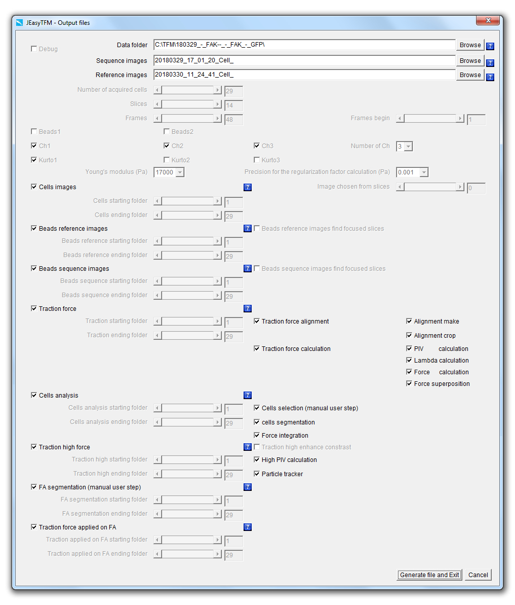
    Generate_file_and_Exit: The button will validate the selections within the JEasyTFM>Create_job window, save the data of the analysis configuration job into a batch file (JEasy.txt) within the ImageJ plugins folder and close the JEasyTFM>Create_job window.

    Cancel: The button will cancel the selections within the JEasyTFM>Create_job window, without saving the data of the analysis configuration job into a batch file (JEasy.txt) and close the JEasyTFM>Create_job window.


    JEasyTFM - Input and output files and folders names and formats (pdf version) [top]


    Output_files_GUI Output Data Folder Output Sequence images Output Reference images Output Cells images Output Beads reference images Output Beads sequence images Output Traction force Output Traction force alignment Output Alignment make Output Alignment crop Output Traction force calculation Output PIV calculation Output lambda calculation Output Force calculation Output Force superposition Output Cells analysis Output Cells selection Output Cells segmentation Output Force integration Output Traction high force Output High PIV calculation Output Particle tracker Output FA segmentation Output Traction force applied on FA Output Generate file and Exit Cancel

    Data formats and folders of the images to be analyzed [top]

    For a TFM time-lapse experiment, z-stack and time-series images need to be gathered for each acquired channel (within them need at least to be a bead and cell image) and xy position (i.e. cell).
    Once the time-series images are acquired, z-stack images of the beads at equilibrium (named reference images later in this document) need to be taken as well for each xy position.
    The input files must be in OME TIF format with the z-stack (slices) images followed by the t-series (frames) images within a single file.
    Each xy stage position (corresponding to a cell) and channel have to be saved within a single file.
    Additionally, the filenames need to finish with the cell number as a string followed by an underscore (i.e. "_") and an iterated channel number padded to two digits (i.e. the images for the cell 1 with 3 acquired channels will finish with "1_01.tif", "1_02.tif" and "1_03.tif").
    For example for the cell number 12 with 3 acquired channels, the filenames should finish with:
    • 12_34.tif
    • 12_35.tif
    • 12_36.tif
    The numbers 34, 35 and 36 being respectively calculated with the equation:
    • [3 × (cell_number − 1) + channel_number]
    which gives for our taken example of the cell number 12 respectively the values:
    • [3 × (12 − 1) + 1] = 34
    • [3 × (12 − 1) + 2] = 35
    • [3 × (12 − 1) + 3] = 36
    The Beads_Reference_images of a given experiment need to be saved within a folder having the same name than the one of the kinetic acquisition followed by _-_Reference.
    The conditions on the filenames and formats are similar to the one described for the kinetic acquisition images.

    Data folder and file names definitions [top]

    If we have for example image filenames for the cell number 12 being:
    • ProtocolCombination_14.11.2018_15_51_21_Cell_12_34.tif
    • ProtocolCombination_14.11.2018_15_51_21_Cell_12_35.tif
    • ProtocolCombination_14.11.2018_15_51_21_Cell_12_36.tif
    we define as prefixes the beginning of the filename that has to be defined in the text field File or Reference_images as described below.
    In the example, this will be:
      ProtocolCombination_14.11.2018_15_51_21_Cell_
    given that the ends of the filenames
    • 12_34.tif
    • 12_35.tif
    • 12_36.tif
    are automatically deduced by the algorithm.

    Job files backups [top]

    Each time a job is launched, a copy of the job file "JEasyTFM.txt" file (saved in the "ImageJ/plugins" folder) used for the given launch is saved in a folder named "jobs" with the name "JEasyTFM_y_begin.txt"; y corresponding to the number of launches made. This means that on the first job launch within the given experiment folder, the copied job name will be "JEasyTFM_1_begin.txt", on the second launch it will be "JEasyTFM_2_begin.txt" and so on, giving thus traceability of the different launches made.
    On top of this, each time an analysis section or iteration for a cell number or folder within a section is completed, an updated version of the job file (i.e. corresponding to the analysis that needs still to be performed) is saved in the "jobs" folder with the name "JEasyTFM_y_end.txt"; y corresponding to the given number of launch made. Thus in the case a job has been stopped or canceled before completion, the user has just to overwrite the "JEasyTFM.txt" file within the "ImageJ/plugins" folder by the "JEasyTFM_y_end.txt" file saved within the "jobs" folder to restart the last job where it had been stopped or canceled.

    Cells images extraction output files [top]

    Cells images extraction Output Cells images
    The Cells_images analysis creates a folder for each cell number defined within Cells_starting_folder and Cells_ending_folder within which all following analysis data will be saved.
    In this part of the analysis, the best focused images for all the frames of the acquired channels for all the acquired cells will be extracted.
    The outputted images will be named
    • Cells_Ch1_xx.tif
    • Cells_Ch2_xx.tif
    • Cells_Ch3_xx.tif
    depending on the channel they represent and
    • Cells_xx.tif
    in the case there is only one acquired channel; xx corresponding to the given frame of the time series.
    The images will be saved in a folder named Cell z; z corresponding to the given cell number.

    Beads reference images best focus extraction output files [top]

    Beads reference images extraction Output Beads reference images

    In this part of the analysis the best focused images of the beads at equilibrium (i.e. after the addition of trypsin also called reference images) for all the acquired cells will be extracted.
    The extracted images will be named
      BeadsReference.tif.
    In the case of the activation of the checkbox
      Beads1
    the images will be named
      BeadsReference_1.tif
    and in the case of the activation of the checkbox
      Beads2
    the images will be named
      BeadsReference_2.tif.
    The images will be saved in a folder named Cell z; z corresponding to the given cell number.

    Beads sequence images best focus extraction output files [top]

    Beads images extraction Output Beads sequence images

    In this part of the analysis the best focused images for all the frames of the beads for all the acquired cells will be extracted.
    The images will be named
      BeadsAfter_xx.tif; xx corresponding to the given frame of the time series.
    In the case of the activation of the checkbox
      Beads1
    the images will be named
      BeadsAfter_1_xx.tif
    and in the case of the activation of the checkbox
      Beads2
    the images will be named
      BeadsAfter_2_xx.tif.
    The images will be saved in a folder named
      Cell z; z corresponding to the given cell number.

    Traction force analysis output files [top]

    Traction force output Output Traction force Output Traction force alignment Output Alignment make Output Alignment crop Output Traction force calculation Output PIV calculation Output lambda calculation Output Force calculation Output Force superposition

    In this section of the package, the main features of the traction force analysis will be performed divided into different sections.

    Traction force alignment output files: The Traction_force_alignment part of the analysis is composed of an Alignment_make section which aligns the best focused images for all the frames of the beads taking as reference the best focused image of the beads at equilibrium and this for all the acquired cells.
    The translation of images with respect to the reference image done by the Alignment_make section will introduce borders that have to be eliminated.
    To do so, the Alignment_crop section opens the images of the beads, measure the position of the borders and crop them out.
    Finally the images of the beads created by the Alignment_make algorithm will be overwritten.
    Similarly, all the images of the cells created by the previous algorithm are opened, cropped and overwritten.

    Alignment make output files: The Alignment_make section aligns the best focused images for all the frames of the beads taking as reference the best focused image of the beads at equilibrium and this for all the acquired cells.
    The output images will be named
    • CorrBeadsAfter_xx.tif; xx corresponding to the given frame of the time series
    and saved in a folder named
    • Cell z/CorrBeadsAfter; z corresponding to the given cell number.
    In the case of the activation of the checkbox
      Beads1
    the images will be named
    • CorrBeadsAfter_1_xx.tif
    and saved in a folder named
    • Cell z/CorrBeadsAfter_1
    In the case of the activation of the checkbox
      Beads2
    the images will be named
    • CorrBeadsAfter_2_xx.tif
    and saved in a folder named
    • Cell z/CorrBeadsAfter_2
    The images of the beads at equilibrium for all the acquired cells will be named
    • CorrBeadsReference.tif
    and saved in a folder named
    • Cell z/Analysis
    together with a file named
    • Transformation.txt
    which records the x and y translation values that have been applied between the
    • BeadsAfter_xx.tif
    and
    • CorrBeadsAfter_xx.tif
    images.
    In the case of the activation of the checkbox
      Beads1
    the reference images will be named
    • CorrBeadsReference_1.tif
    and saved in a folder named
    • Cell z/Analysis_1
    together with the
    • Transformation.txt
    file.
    In the case of the activation of the checkbox
      Beads2
    the reference images will be named
    • CorrBeadsReference_2.tif
    and saved in a folder named
    • Cell z/Analysis_2
    together with the
    • Transformation.txt
    file.
    The translation transformations that have been applied on the
    • CorrBeadsAfter_xx.tif
    images (and saved in the Transformation.txt file) are similarly applied on the best focused images for all the frames of the acquired channels for all the acquired cells.
    The outputted images will be named
    • CorrCells_Ch1_xx.tif
    • CorrCells_Ch2_xx.tif
    • CorrCells_Ch3_xx.tif
    depending on the channel they represent and
    • CorrCells_xx.tif
    in the case there is only one acquired channel and saved in a folder named
    • Cell z/CorrCells
    In the case of the activation of the checkbox
      Beads1
    the images will be named
    • CorrCells_1_Ch1_xx.tif
    • CorrCells_1_Ch2_xx.tif
    • CorrCells_1_Ch3_xx.tif
    depending on the channel they represent and
    • CorrCells_1_xx.tif
    in the case there is only one acquired channel and saved in a folder named
    • Cell z/CorrCells_1
    In the case of the activation of the checkbox
      Beads2
    the images will be named
    • CorrCells_2_Ch1_xx.tif
    • CorrCells_2_Ch2_xx.tif
    • CorrCells_2_Ch3_xx.tif
    depending on the channel they represent and
    • CorrCells_2_xx.tif
    in the case there is only one acquired channel and saved in a folder named
    • Cell z/CorrCells_2

    Alignment crop output files: The translation of images with respect to the reference image done by the Alignment_make section will introduce borders that have to be eliminated.
    To do so, the Alignment_crop section opens the images of the beads, measures the position of the borders, crops them out and adds the border positions data to the previously generated Transformation.txt file.
    Finally the images of the beads created by the Alignment_make algorithm will be overwritten.
    Similarly, all the images of the cells created by the previous algorithm are opened, cropped and overwritten.

    Traction force calculation output files: The Traction_force_calculation part of the analysis is composed of a PIV_calculation section which applies a PIV (Particle Image Velocimetry) algorithm between the reference images of the beads and the images for all the frames of the beads generated at the Traction_force_alignment section.
    Next, the Force_calculation section will generate the corresponding force maps using a FTTC (Fourier Transform Traction Cytometry) algorithm.
    And the Force_superposition section will combine all the cells with all the force maps images.

    PIV calculation output files: The PIV_calculation section which will apply a PIV (Particle Image Velocimetry) algorithm between the reference images of the beads and the images for all the frames of the beads generated at the Traction_force_alignment section.
    The results are outputted in the form of text in a file named
    • Stack_xx.txt; xx corresponding to the given frame of the time series
    together with a image representing the beads displacement magnitude and vectors named
    • PIV3_Stack_xx.tif
    and saved in a folder named
    • Cell z/Analysis; z corresponding to the given cell number.
    In the case of the activation of the checkbox
      Beads1
    the output files will be named
    • Stack_1_xx.txt
    and
    • PIV3_Stack_1_xx.tif
    and saved in a folder named
    • Cell z/Analysis_1.
    In the case of the activation of the checkbox
      Beads2
    the output files will be named
    • Stack_2_xx.txt
    and
    • PIV3_Stack_2_xx.tif
    and saved in a folder named
    • Cell z/Analysis_2.

    Lambda calculation output files: The Lambda_calculation section will read all the previously generated
    • Stack_xx.txt; xx corresponding to the given frame of the time series
    files and determine the regularization or Lagrange parameter λ value so that the calculated force maps using an FTTC (Fourier Transform Traction Cytometry) algorithm will stand within the Precision_for_the_Regularization_factor_calculation value of the optimal force and this for all Frames.
    The results are outputted in the form of text in a file named
    • lambda.txt
    saved in a folder named
    • Cell z/Analysis; z corresponding to the given cell number.
    In the case of the activation of the checkbox
      Beads1
    the file will be saved in a folder named
    • Cell z/Analysis_1.
    In the case of the activation of the checkbox
      Beads2
    the file will be saved in a folder named
    • Cell z/Analysis_2.

    Force calculation output files: The Force_calculation section first reads all the previously generated
    • Stack_xx.txt; xx corresponding to the given frame of the time series
    files and generates all the corresponding force maps using an FTTC (Fourier Transform Traction Cytometry) algorithm to evaluate the minimal and maximal values of the obtained force vectors.
    These values are then stored in a text file named
    • scale.txt
    and saved in the folder
    • Cell z/Analysis; z corresponding to the given cell number.
    Following the obtained maximal value is ceil rounded by a 'nice number' and used for defining the maximum force vector value so that the force scaling is normalized through the whole acquired images.
    The obtained force outputs are then saved in a text file named
    • Traction_Stack_xx.txt
    in the folder
    • Cell z/Analysis.
    The images of the vector and magnitude maps are named
    • Traction_Vector_Plot_Traction_Stack_xx.tif
    and
    • Traction_Magnitude_Plot_Traction_Stack_xx.tif
    and saved in a folder named
    • Cell z/Traction_Vector_Plot.
    In the case of the activation of the checkbox
      Beads1
    the output files will be named
    • scale_1.txt
    and
    • Traction_Stack_1_xx.txt
    and saved in the folder
    • Cell z/Analysis_1.
    as well as
    • Traction_Vector_Plot_Traction_Stack_1_xx.tif
    and
    • Traction_Magnitude_Plot_Traction_Stack_1_xx.tif
    which are saved in a folder named
    • Cell z/Traction_Vector_Plot_1.
    In the case of the activation of the checkbox
      Beads2
    the output files will be named
    • scale_2.txt
    and
    • Traction_Stack_2_xx.txt
    and saved in the folder
    • Cell z/Analysis_2
    as well as
    • Traction_Vector_Plot_Traction_Stack_2_xx.tif
    and
    • Traction_Magnitude_Plot_Traction_Stack_2_xx.tif
    which are saved in a folder named
    • Cell z/Traction_Vector_Plot_2

    Force superposition output files: The Force_superposition section will combine all the cells with all the force maps images.
    Thus the outputted images will be named:
    • Superposition_with_Traction_Vector_Plot_Ch1_xx.jpg
    • Superposition_with_Traction_Magnitude_Plot_Ch1_xx.jpg; xx corresponding to the given frame of the time series
    or
    • Superposition_with_Traction_Vector_Plot_Ch2_xx.jpg
    • Superposition_with_Traction_Magnitude_Plot_Ch2_xx.jpg
    or
    • Superposition_with_Traction_Vector_Plot_Ch3_xx.jpg
    • Superposition_with_Traction_Magnitude_Plot_Ch3_xx.jpg
    depending on the channel they represent and:
    • Superposition_with_Traction_Vector_Plot_xx.jpg
    • Superposition_with_Traction_Magnitude_Plot_xx.jpg
    in the case there is only one acquired channel and saved in a folder named
    • Cell z/PicCells; z corresponding to the given cell number.
    In the case of the activation of the checkbox
      Beads1
    the images will be named:
    • Superposition_with_Traction_Vector_Plot_1_Ch1_xx.jpg
    • Superposition_with_Traction_Magnitude_Plot_1_Ch1_xx.jpg
    or
    • Superposition_with_Traction_Vector_Plot_1_Ch2_xx.jpg
    • Superposition_with_Traction_Magnitude_Plot_1_Ch2_xx.jpg
    or
    • Superposition_with_Traction_Vector_Plot_1_Ch3_xx.jpg
    • Superposition_with_Traction_Magnitude_Plot_1_Ch3_xx.jpg
    depending on the channel they represent and:
    • Superposition_with_Traction_Vector_Plot_1_xx.jpg
    • Superposition_with_Traction_Magnitude_Plot_1_xx.jpg
    in the case there is only one acquired channel and saved in a folder named
    • Cell z/PicCells_1.
    In the case of the activation of the checkbox
      Beads2
    the images will be named:
    • Superposition_with_Traction_Vector_Plot_2_Ch1_xx.jpg
    • Superposition_with_Traction_Magnitude_Plot_2_Ch1_xx.jpg
    or
    • Superposition_with_Traction_Vector_Plot_2_Ch2_xx.jpg
    • Superposition_with_Traction_Magnitude_Plot_2_Ch2_xx.jpg
    or
    • Superposition_with_Traction_Vector_Plot_2_Ch3_xx.jpg
    • Superposition_with_Traction_Magnitude_Plot_2_Ch3_xx.jpg
    depending on the channel they represent and:
    • Superposition_with_Traction_Vector_Plot_2_xx.jpg
    • Superposition_with_Traction_Magnitude_Plot_2_xx.jpg
    in the case there is only one acquired channel and saved in a folder named
    • Cell z/PicCells_2.

    Cells analysis output files [top]

    Cells analysis output Output Cells analysis Output Cells selection Output Cells segmentation Output Force integration
    In the Cells_analysis part of the analysis, the segmentation of the images of the cells as well as the force integration over the cells over all the frames will be performed.
    The Cells_segmentation part of the analysis applies several filters to the acquired images of the cells and the Cells_selection part of the analysis requires the user to draw a ROI (Region Of Interest) delimiting the displacements of the cell of interest over all the frames as well as to define a threshold window for the given cell over all the frames in order to generate cells segmentation ROIs.
    The Force_integration part of the analysis makes a superposition of the different cell images together with the vector and magnitude force representations images and the cell ROI together with the measured integrated values.

    Cells selection output files: The Cells_selection part of the analysis requires the user to draw a ROI (Region Of Interest) delimiting the displacements of the cell of interest over all the frames as well as to define a threshold window for the given cell over all the frames.
    The output will be a ROI file for all the frames named
    • RoiSet.zip
    and saved in the folder
    • Cell z/Analysis.
    As well as a stack image named
    • segmentation.tif
    and saved in the folder
    • Cell z
    that is a superposition of the images of the cells will all the calculated ROIs.
    In the case of the activation of the checkbox
      Beads1
    the output ROI file
    • RoiSet.zip
    will be saved in the folder
    • Cell z/Analysis_1
    and in the case of the activation of the checkbox
      Beads2
    it will be saved in the folder
    • Cell z/Analysis_2.

    Cells segmentation output files: The Cells_segmentation part of the analysis applies several filters to the acquired images of the cells and output images named
    • focused.tif
    and
    • binaries.tif
    that are saved in the folder
    • Cell z; z corresponding to the given cell number.
    This intermediate step aims to reduce the waiting time for the user between the analyses of each cell through the final segmentation algorithm that will have manual steps.

    Force integration output files:
    The Force_integration part of the analysis makes a copy of the previous PIV output text file
    • Stack_xx.txt; xx corresponding to the given frame of the time series
    in a folder named
    • Cell z/Integration_calculation; z corresponding to the given cell number
    and generates similarly to the Force_calculation section all the files generated by the FTTC algorithm, i.e.:
    • Traction_Stack_xx.txt
    • Traction_Vector_Plot_Traction_Stack_xx.tif
    • Traction_Magnitude_Plot_Traction_Stack_xx.tif
    • Traction_Vector_Scale.tif
    in the same folder.
    The generation of all these files in a new folder may be redundant, but it is a very fast process and above all, it is able to compartmentalize the creation of
    • Plot_Traction
    images on which the parameters can be played around in order for example to increase or decrease the vector lengths or relative intensity for the superimposed images generated at the next section.
    In the case of the activation of the checkbox
      Beads1
    the files will be named
    • Stack_1_xx.txt
    • Traction_Stack_1_xx.txt
    • Traction_Vector_Plot_Traction_Stack_1_xx.tif
    • Traction_Magnitude_Plot_Traction_Stack_1_xx.tif
    • Traction_Vector_Scale.tif
    and saved in a folder named
    • Cell z/Integration_calculation_1.
    In the case of the activation of the checkbox
      Beads2
    the files will be named
    • Stack_2_xx.txt
    • Traction_Stack_2_xx.txt
    • Traction_Vector_Plot_Traction_Stack_2_xx.tif
    • Traction_Magnitude_Plot_Traction_Stack_2_xx.tif
    • Traction_Vector_Scale.tif
    and saved in a folder named
    • Cell z/Integration_calculation_2.

    Next the superposition of the different cell images together with the vector and magnitude force representations images and the cell ROI as well as measured integrated values are generated and named
    • Integration_with_Traction_Vector_Plot_Ch1_xx.jpg
    • Integration_with_Traction_Magnitude_Plot_Ch1_xx.jpg; xx corresponding to the given frame of the time series
    or
    • Integration_with_Traction_Vector_Plot_Ch2_xx.jpg
    • Integration_with_Traction_Magnitude_Plot_Ch2_xx.jpg
    or
    • Integration_with_Traction_Vector_Plot_Ch3_xx.jpg
    • Integration_with_Traction_Magnitude_Plot_Ch3_xx.jpg
    depending on the channel they represent and:
    • Integration_with_Traction_Vector_Plot_xx.jpg
    • Integration_with_Traction_Magnitude_Plot_xx.jpg
    in the case there is only one acquired channel and saved in a folder named
    • Cell z/Integration_results; z corresponding to the given cell number.
    In the case of the activation of the checkbox
      Beads1
    the images will be named:
    • Integration_with_Traction_Vector_Plot_1_Ch1_xx.jpg
    • Integration_with_Traction_Magnitude_Plot_1_Ch1_xx.jpg
    or
    • Integration_with_Traction_Vector_Plot_1_Ch2_xx.jpg
    • Integration_with_Traction_Magnitude_Plot_1_Ch2_xx.jpg
    or
    • Integration_with_Traction_Vector_Plot_1_Ch3_xx.jpg
    • Integration_with_Traction_Magnitude_Plot_1_Ch3_xx.jpg
    depending on the channel they represent and:
    • Integration_with_Traction_Vector_Plot_1_xx.jpg
    • Integration_with_Traction_Magnitude_Plot_1_xx.jpg
    in the case there is only one acquired channel and saved in a folder named
    • Cell z/Integration_results_1.
    In the case of the activation of the checkbox
      Beads2
    the images will be named:
    • Integration_with_Traction_Vector_Plot_2_Ch1_xx.jpg
    • Integration_with_Traction_Magnitude_Plot_2_Ch1_xx.jpg
    or
    • Integration_with_Traction_Vector_Plot_2_Ch2_xx.jpg
    • Integration_with_Traction_Magnitude_Plot_2_Ch2_xx.jpg
    or
    • Integration_with_Traction_Vector_Plot_2_Ch3_xx.jpg
    • Integration_with_Traction_Magnitude_Plot_2_Ch3_xx.jpg
    depending on the channel they represent and:
    • Integration_with_Traction_Vector_Plot_2_xx.jpg
    • Integration_with_Traction_Magnitude_Plot_2_xx.jpg
    in the case there is only one acquired channel and saved in a folder named
    • Cell z/Integration_results_2.

    All the integration data are resumed in a table saved in a text file named
    • Integration_results.txt
    and saved in the folder
    • Cell z.

    Beads positions tracking output files [top]

    Traction high force output Output Traction high force Output High PIV calculation Output Particle tracker
    In the Traction_high_force part of the analysis, the tracking of the beads between the reference images of the beads and the images for all the frames of the beads generated at the Traction_force_alignment section will be performed.
    The Traction_high_force part of the analysis is composed of a High_PIV_calculation section which takes the data previously obtained from the PIV_calculation section of the Traction_force_calculation part of the analysis to push the calculation further to have a more refined definition of the beads displacement map.
    The Particle_tracker section will use the more refined definition of the beads displacement map to compute the displacement of the beads.

    High PIV calculation output files: The High_PIV_calculation section which will take the data previously obtained from the PIV_calculation section of the Traction_force_calculation part of the analysis, saved in the
    • Stack_xx.txt; xx corresponding to the given frame of the time series
    file to push the calculation further to have a more refined definition of the beads displacement map.
    The results are outputted in the form of text in a file named
    • Stack_xx_2.txt
    and saved in the folder
    • Cell z/Analysis; z corresponding to the given cell number.
    In the case of the activation of the checkbox
      Beads1
    the output files will be named
    • Stack_1_xx_2.txt
    and saved in the folder
    • Cell z/Analysis_1.
    And in the case of the activation of the checkbox
      Beads2
    the output files will be named
    • Stack_2_xx_2.txt
    and saved in the folder named
    • Cell z/Analysis_2.

    Particle tracker output files: The Particle_tracker section uses the previously generated
    • Stack_xx_2.txt; xx corresponding to the given frame of the time series
    file in order to compute the displacement of the beads.
    The obtained outputs are saved in a text file named
    • Stack_xx_2_Trajectories.txt
    in the folder
    • Cell z/Analysis; z corresponding to the given cell number.
    As the images of the beads displacements they are named
    • Stack_xx_Trajectories.tif
    and saved in a folder named
    • Cell z/Trajectories.
    In the case of the activation of the checkbox
      Beads1
    the output files will be named
    • Stack_1_xx_2_Trajectories.txt
    and saved in the folder
    • Cell z/Analysis_1
    as well as
    • Stack_1_xx_Trajectories.tif
    and saved in a folder named
    • Cell z/Trajectories_1.
    And in the case of the activation of the checkbox
      Beads2
    the output files will be named
    • Stack_2_xx_2_Trajectories.txt
    and saved in the folder
    • Cell z/Analysis_2
    as well as
    • Stack_2_xx_Trajectories.tif
    and saved in a folder named
    • Cell z/Trajectories_2.

    FA segmentation output files [top]

    FA segmentation output Output FA segmentation
    Within the FA_segmentation section, a segmentation of focal adhesion algorithm outputs a ROI file named
    • RoiSet_xx.zip; xx corresponding to the given frame number.
    as well as a stack image named
    • CorrCells_xx.tif
    and saved in the folder
    • Cell z/FA_Analysis; z corresponding to the given cell number.
    In the case of the activation of the checkbox
      Beads1
    the files will be named
    • RoiSet_1_xx.zip
    • CorrCells_1_xx.tif
    and saved in a folder named
    • Cell z/FA_Analysis_1.
    In the case of the activation of the checkbox
      Beads2
    the files will be named
    • RoiSet_2_xx.zip
    • CorrCells_2_xx.tif
    and saved in a folder named
    • Cell z/FA_Analysis_2.

    Traction force applied on FA output files [top]

    Traction force applied on FA output Output Traction force applied on FA
    The Traction_force_applied_on_FA7-10 algorithm outputs
    text files named
    • FA_positions_xx.txt
    • Beads_displacements_xx.txt
    • Fitting_parameters_data_xx.tif
    and images named
    • Beads_displacement_plot_xx.tif
    • Beads_displacement_plot_with_image_xx.tif
    • Regularization_parameter_plot_xx.tif
    • Force_plot_xx.tif
    • Force_plot_with_image_xx.tif; xx corresponding to the given frame of the time series
    and saved in the folder
    • Cell z/Traction_force_on_FA; z corresponding to the given cell number.
    If the checkboxes Ch1 and/or Ch2 and/or Ch3 is/are activated, this algorithm will then be applied to the beads displacements and FA positions data merge of all the selected beads colors.

     (7) Balaban, N. Q., Schwarz, U. S., Riveline, D., Goichberg, P., Tzur, G., Sabanay, I., Mahalu, D., Safran, S., Bershadsky, A., Addadi, L. and Geiger, B.
      Force and focal adhesion assembly: a close relationship studied using elastic micro-patterned substrates. Nat. Cell Biol. 3, 466-472 (2001)
     (8) Schwarz, U. S., Balaban, N. Q., Riveline, D. Bershadsky, A., Geiger, B., Safran, S. A.
      Calculation of forces at focal adhesions from elastic substrate data: the effect of localized force and the need for regularization, Biophys. J. 83, 1380-1394 (2002)
     (9) Schwarz, U. S., Balaban, N. Q., Riveline, D., Addadi, L., Bershadsky, A., Safran, S. A., Geiger, B.
      Measurement of cellular forces at focal adhesions using elastic micro-patterned substrates, Mat. Sci. Eng. C 23, 387-394 (2003)
    (10) Sabass, B., Gardel, M. L., Waterman, C. and Schwarz, U. S.
      high-resolution traction force microscopy based on experimental and computational advances, Biophys. J., 94,207-220, (2008)


    Technical requirements for the use of JeasyTFM [top]


    Beads Displacement [top]

    The gel deformation is measured by the technique of PIV (Particle Image Velocytometry) which measure the change of beads spatial position between constrained and unconstrained conditions and thus tracks the fluorescent beads in different interrogation windows. Therefore, the accuracy of this method is dependent upon parameters such as (1) the number of beads per image, (2) the signal to noise ratio of the images of the beads and (3) the precision of the bead tracking algorithm.

    1 - Minimal number of beads per images [top]

    The number of beads within the images is as well an important parameter to consider in order to properly reconstruct the traction force maps exerted by the cells on a surface. To determine the lower bead density required for traction force reconstruction within JEasyTFM, we tested images with different beads density. We started with a low bead density of 3000 beads for a 1124 × 1164 pixels image, and then artificially decreased the number of the beads of the reference and sequence images of the beads. Note that the acquired original images had a size of 1200 × 1200 pixels which have been slightly reduced through the Traction force alignment algorithm (i.e. Alignment make and Alignment crop). To do so, the intensity of circular ROIs of 10 pixels centered at the positions of the beads was set to the intensity value of the background. The choice of the beads to be erased in the reference and sequence images had then been chosen using a random number generator. The figure below shows force maps images obtained for different beads density. As expected, decreasing the beads density to 2500 beads / 1124 × 1164 pixels decreases the resolution of the traction force reconstruction map (compare figure 3000 beads with 2000 beads) without altering the overall reconstruction map. However, reducing the bead density to 1500 beads / 1124 × 1164 pixels clearly starts to alter the traction force reconstruction map. Please note that by dragging the mouse over the force maps images, the image is replaced by a movie illustrating the switch between the two images of the beads (i.e. before and after addition of Reference) that have been used to generate the given force map. These movies clearly show the diminution of the beads density.

    S/N = 3.4153 ± 0.9159 S/N = 2.3005 ± 0.5999
    3000 beads 2500 beads


    S/N = 2.1002 ± 0.5073 S/N = 2.0005 ± 0.4576
    2000 beads 1500 beads


    S/N = 1.9501 ± 0.2813 S/N = 1.9003 ± 0.2625
    1000 beads 500 beads

    2 - Minimal signal to noise ratio of the images of the beads [top]

    Given that the positions of the beads are the fiducial markers used to reconstruct the traction forces exerted by the cells on their support, it is mandatory to acquire images of the beads by respecting a minimum signal to noise ratio value. To evaluate this number, we first measured the mean and standard deviation of the signal-to-noise ratio of the images of the beads by calculating the mean and standard deviation of the intensity ratio integrated over all the images of an experiment (i.e. all stack-z and time-series images). Depending on the system used to acquire the images of the beads, we found a signal-to-noise ratio value up to 7 for the best system we tested and in the chosen example (see below) we measured a signal to noise ratio of 3.4153 ± 0.9159. To test the output results of the force reconstruction algorithm with images having lower signal to noise ratio values, we artificially degraded their quality by using an Enhance Contrast filter with different Saturated pixels values. The figure below shows force maps images obtained for images of the beads having different values of the signal-to-noise ratio. We notice that there is no degradation within the force maps resolution until a signal-to-noise ratio value lower than 2. Please note that by dragging the mouse over the force maps images, the image is replaced by a movie illustrating the switch between the two images of the beads (i.e. before and after addition of trypsin) that have been used to generate the given force map. These movies clearly show the alteration of the beads signal upon applying the Enhance Contrast filter.

    S/N = 3.4153 ± 0.9159 S/N = 2.3005 ± 0.5999
    S/N = 3.4153 ± 0.9159 S/N = 2.3005 ± 0.5999


    S/N = 2.0005 ± 0.4576 S/N = 1.9003 ± 0.2625
    S/N = 2.0005 ± 0.4576 S/N = 1.9003 ± 0.2625


    S/N = 1.7001 ± 0.2173 S/N = 1.1006 ± 0.1549
    S/N = 1.7001 ± 0.2173 S/N = 1.1006 ± 0.1549

    3a - Bead tracking - Build upon the Particle_Tracker 1.5. version released September 2006 [top]

    The ParticleTracker_2D code developed by the MOSAIC group and published in:
    was used as a starting point for the bead tracking routine.

    We did not change the first part of the code, which is used for "Particle detection". The "Particle linking" part of the code using a Particle Tracking Velocimetry (PTV) method is used to track the displacement of the beads between strained and unstrained positions. This part of the code is based on scoring between the differences of the positions of the beads, grey values and derivations of the grey values upon the definition of a “Displacement” value (see Figure below).

    ParticleTracker_2D GUI ParticleTracker_2D GUI
    Graphical User Interface of the original ParticleTracker_2D plugin with on left the interface before launching the algorithm and on right the one obtained after the tracking completed

    However, the setting of a "Displacement" value does not always allow an accurate tracking of the beads over the whole image. In fact, beads couples (i.e. the associations of the same bead in the reference and given sequence image) displaying large displacements will be missed if the displacement value has been set to a value that is smaller than the largest bead displacement found in the image. Moreover, if the displacement value has been set to a value equal or higher to the largest bead displacement, the algorithm then generates often wrong beads couples associations. This is well documented in the Figures below, which show results obtained with the original ParticleTracker_2D plug-in using different "Displacement" values within the plugin GUI. As observed when the displacement value is set to 5 pixels, some of the large bead displacements are not taken into account (green circle), whereas when the displacement value is set to 15 pixels, wrong beads couple association can be observed (blue circle).

    Displacement = 5 pixels Displacement = 10 pixels
    ParticleTracker_2D output with Displacement set to 5 pixels ParticleTracker_2D output with Displacement set to 10 pixels


    Displacement = 15 pixels Displacement = 20 pixels
    ParticleTracker_2D output with Displacement set to 15 pixels ParticleTracker_2D output with Displacement set to 20 pixels

    To improve the quality of the beads tracking routine, we modified the original ParticleTracker_2D algorithm by implementing the results of the displacements maps obtained by the PIV algorithm as starting positions for the tracking algorithm. This allows to use a minimal displacement value and thus eliminate all wrong beads couples associations. The use of a small displacement value requires using a displacement map with a small grid size of 8 pixels. The Figures below show results obtained with our Particle_Tracker_PIV_and_Trajectories_Inputs plugin implemented within JEasyTFM using as input a PIV calculation map with a grid size of 8 pixels and "Displacement" value set to 5 within the plugin GUI.

    ParticleTracker_2D GUI ParticleTracker_2D GUI
    Graphical User Interface of our Particle_Tracker_PIV_and_Trajectories_Inputs plugin with on left the interface before launching the algorithm and on right the one obtained after the tracking completed.
    PIV calculation with a grid size of 8 pixels Displacement = 5 pixels
    PIV calculation with a grid size of 8 pixels Particle_Tracker_PIV_and_Trajectories_Inputs output with Displacement set to 5 pixels
    ParticleTracker_2D GUI ParticleTracker_2D GUI
    Graphical User Interface of the original Particle_Tracker_2D/3D tool of the MosaicSuite package with on left the interface before launching the algorithm and on right the one obtained after the tracking completed

    Similarly, the setting of a "Displacement" value does not always allow an accurate tracking of the beads over the whole image, either missing large displacements or generating wrong beads couples associations. This is shown within the Figures below, which show results obtained with the original Particle_Tracker_2D/3D tool plug-in using different "Displacement" values within the plugin GUI. As observed when the displacement value is set to 5 pixels, some of the large bead displacements are not taken into account (green circle), whereas when the displacement value is set to 15 pixels, wrong beads couple association can be observed (blue circle).

    Displacement = 5 pixels Displacement = 10 pixels
    Particle_Tracker_2D/3D tool output with Displacement set to 5 pixels Particle_Tracker_2D/3D tool output with Displacement set to 10 pixels


    Displacement = 15 pixels Displacement = 20 pixels
    Particle_Tracker_2D/3D tool output with Displacement set to 15 pixels Particle_Tracker_2D/3D tool output with Displacement set to 20 pixels

    To improve the quality of the beads tracking routine, we modified the original Particle_Tracker_2D/3D tool algorithm by implementing the results of the displacements maps obtained by the PIV algorithm as starting positions for the tracking algorithm. This allows to use a minimal displacement value and thus eliminate all wrong beads couples associations. The use of a small displacement value requires using a displacement map with a small grid size of 8 pixels. The Figures below show results obtained with our MosaicSuite-1.0.25_Full_extended package update implemented within JEasyTFM using as input a PIV calculation map with a grid size of 8 pixels and "Displacement" value set to 5 within the plugin GUI.

    ParticleTracker_2D GUI ParticleTracker_2D GUI
    Graphical User Interface of our Particle_Tracker_2D/3D tool within our MosaicSuite-1.0.25_Full_extended package update with on left the interface before launching the algorithm and on right the one obtained after the tracking completed
    PIV calculation with a grid size of 8 pixels Displacement = 5 pixels
    PIV calculation with a grid size of 8 pixels Particle_Tracker_2D/3D tool using the PIV outputs with Displacement set to 5 pixels

    Traction force reconstruction [top]

    The reconstruction routine used in JeasyTFM provides (1) the Extended Depth of Field plugin to extract the best focused images of the beads for both the reference and all the sequence images and (2) the possibility to run the Find focused slices plugin prior launching the Extended Depth of Field plugin to reduce the number of z-slices images.

    In addition, the traction force reconstruction routine used in JeasyTFM is mainly based on the one published in Martiel, J.-L. et al. (2015) Measurement of cell traction forces with ImageJ. Methods Cell Biol., 125, 269–287, which used the Fourier Transform Traction Cytometry (FTTC) method to measure the traction force exerted by the cell inducing the gel deformation and bead displacement. The original code was simplified and improved. Maps, exporting LUTs and style possibilities such as "Draw magnitude and vector", Draw X magnitude" and "Draw Y magnitude" were added. The force maps can also now be generated in Newtons and/or in Pascals (versus only in Pa previously). This reconstruction depends mainly on two parameters i.e the grid size value and the regularization factor.

    Original FTTC GUI Modified FTTC GUI
    Graphical User Interface of the original plugin with on the left and on right our updated version.

    1 - Grid size values [top]

    The grid size value is pre-defined in the JeasyTFM plugin. This value can be changed by modifying the source code of the plugin. For the force interpolation, a grid size of 16 pixels was selected which means that the distance between 2 vectors is equal to 16 pixels. The "grid size" has to be a value multiple of 2. Increasing or decreasing this value will either increase or decrease the maps vector spacing and thus decrease or increase the spatial resolution of the traction force map. Below are figures showing PIV calculation maps obtained with different grid size values and the corresponding mean and standard deviation calculation times obtained over 20 runs.

    We pre-defined a grid size value of 16 pixels in JEasy TFM because it is the best compromise between spatial resolution and calculation time. Nevertheless as input for the bead tracking algorithm, used mainly for high-resolution TFM, we use a PIV map generated with a grid size of 8 pixels to be thus able to reduce the allowed beads displacements to 5 pixels.

    Grid size of 64 pixels Grid size of 32 pixels
    Grid size of 64 pixels - Calculation time : 3.97 ± 0.19 s Grid size of 32 pixels - Calculation time : 20.93 ± 0.63 s


    Grid size of 16 pixels Grid size of 8 pixels
    Grid size of 16 pixels - Calculation time : 30.03 ± 1.16 s Grid size of 8 pixels - Calculation time : 181.95 ± 3.52 s

    2 - Regularization factor [top]

    Within the present version of the JEasyTFM GUI, the value of the regularization factor is set through a numeric field with a default choice set to "1.0e-10". To analyzed how the smoothing coefficient affects the value of the forces, we generated 2200 values (i.e. 100 measured values per decade which gives 22 × 100 = 2200 values) of the regularization factor logarithmically distributed between 10-21 and 10 and calculated the corresponding forces (see Figures below).

    The optimal choice for the regularization factor corresponds to the point of inflection of regularization versus force curve. For the example given, this value is ≈ 3.45.10-10.

    Force and force ratio vs regularization factor plots generated for 2200 values of the regularization factor logarithmically distributed between 10-21 and 10.